The framework¶

Runs in PALLADIO are called sessions; a session consists of the execution of all experiments followed by the analysis of the results.

For details on how to perform the experiments and analyze the results, please refer to the Quick start tutorial.

Dataset format¶

A dataset consists of two things:

An input matrix \(X \in \mathbb{R}^{n \times p}\) representing \(n\) samples each one described by \(p\) features; in the case of gene expression microarrays for instance each feature represents
An output vector \({\bf y}\) of length \(n\) whose elements are either a continuous value or a discrete label, describing some property of the samples. These may represent for example the levels of a given substance in the blood of an individual (continuous variable) or the class to which he or she belongs (for instance, someone affected by a given disease or a healthy control).

For the time being, we will only consider a specific instance of the latter case, where the number of classes is two: this is commonly referred to as binary classification scenario.

As previously explained, the core idea behind PALLADIO is to return, together with a list of significant features, not just a single value as an estimate for the prediction accuracy which can be achieved, but a distribution, so that it can be compared with the distribution obtained from experiments when the function is learned from data where the labels have been randomly shuffled (see Introduction).

Pipeline¶

Once the main script has been launched, the configuration file is read in order to retrieve all required information to run all the experiments of a PALLADIO session. These include:

The location of data and labels files.
Experiment design parameters, such as the total number of experiments and the ratio of samples to be used for testing in each experiment.

Parameters specific to the chosen machine learning algorithm: for instance, for the Elastic Net algorithm, the values for the alpha and l1_ratio parameters.

A session folder is created within the folder containing the configuration file, in order to keep everything as contained as possible; data and labels file, together with the configuration file itself, are copied inside this folder. Then, experiments are distributed among the machines of the cluster; each machine will be assigned roughly the same number of jobs in order to balance the load.

Experiments¶

Each experiment is divided in several stages, as shown in Fig. 1:

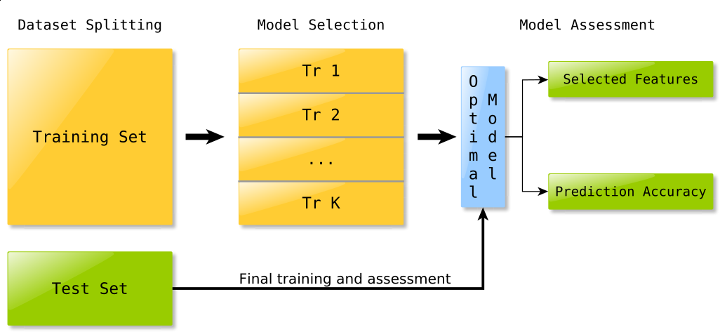
Fig. 1 The stages each experiment goes through.

Dataset split and preprocessing¶

In the very first stage, the dataset is split in training and test set, in a ratio determined by the corresponding parameter in the experiment configuration file; also, during this stage, any kind of data preprocessing (such as centering or normalization) is performed.

Model selection¶

Assuming that the chosen classifier requires some parameter to be specified (for instance the \(\ell_1\) and squared \(\ell_2\) penalities weights when using the \(\ell_1 \ell_2\) regularized least square algorithm), the training set is split in \(K\) chunks (the number \(K\) is also specified in the experiment configuration file) and K-fold cross validation is performed in order to choose the best parameters, that is those which lead to the model with the lowest cross validation error.

Model assessment¶

Finally, the algorithm is trained using the parameters chosen in the previous step on the whole training set; the function obtained is then used to predict the labels of samples belonging to the test set, which have not been used so far in any way, so that the results of whole procedure are unbiased.

At the end of each experiment, results are stored in a .pkl file inside a subfolder whose name will be of the form regular_p_P_i_I for regular experiments and permutation_p_P_i_I for experiments where the training labels have been randomly shuffled, where P and I the process number and within that process a counter which is incremented by one after each experiment.

Analysis¶

The analysis script simply reads the partial results in all experiment folders, consisting of

A list of features
The predicted labels for the test set

With these it computes the accuracy achieved and then uses these elaborated results to produce a number of plots:

Fig. 2 shows the absolute feature selection frequency in both regular experiments and permutation tests; each tick on the horizontal axis represents a different feature, whose position on the vertical axis is the number of times it was selected in an experiment. Features are sorted based on the selection frequency relative to regular experiments; green dots are frequencies for regular experiments, red ones for permutation tests.

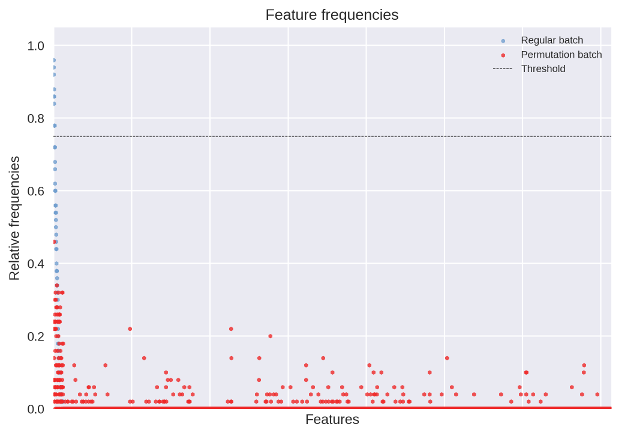
Fig. 2 A manhattan plot showing the distribution of frequencies for both regular experiments and permutation tests.

Fig. 3 shows a detail of the frequeny of the top \(2 \times p_{\rm rel}\) selected features, where \(p_{\rm rel}\) is the number of features identified as relevant by the framework, i.e. those which have been selected enough times according to the selection threshold defined in the configuration file. Seeing the selection frequency of relevant features with respect to the selection frequency of those which have been rejected may help better interpret the obtained results.

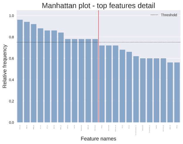
Fig. 3 A detail of the manhattan plot.

Finally, Fig. 4 shows the distribution of prediction accuracies (corrected for class imbalance) for regular experiments and permutation tests; this plot answer the questions:

Is there any signal in the data being analyzed?
If yes, how much the model can describe it?

In the example figure, the two distributions are clearly different, and the green one (showing the accuracies of regular experiments) has a mean which is significantly higher than chance (50 %). A p-value obtained with the Two-sample Kolmogorov–Smirnov test is also present in this plot, indicating whether there is a significant difference between the two distributions.

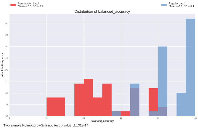
Fig. 4 The distributions of accuracies for both regular experiments and permutation tests.

Results interpretation¶

Once the analysis has been performed, it is possible to draw conclusions from the results of the experiment.

Ideally, in a dataset where there is a significant correlation between input and output, the two distributions of accuracy values will be visibly different, such as those shown in Fig. 4. As a consequenence, the p-value for the Two-sample Kolmogorov–Smirnov test will be very low (see below for more details on the choice of the significance level \(\alpha\)).

The purpose of testing if the two distributions are different is to determine if the feature signature is reliable or not: in facts, if one obtains a poor result in terms of prediction accuracy, there is no point in looking at the list of selected variables, as those would refer to models which were not able to fit the available data.

Significance level¶

When using statistical tests such as the T-test to compare two distributions the p-value is compared with a given threshold or significance level \(\alpha\), which is usually set to 0.05 or 0.01.

However we noticed that, on experiments performed on datasets with no correlation between input and output with the purpose of determining the behaviour of the framework in these cases, the two distributions of accuracy values, albeit being almost identical, yielded a p-value in the order of \(10^{-5}-10^{-4}\). Notice that, being experiments performed on synthetic datasets, we knew in advance that there was no correlation whatsoever and therefore the two distributions had to be indistinguishable.

The suggested significance level when performing 100 experiments per batch (a total of 200) is \(10^{-10}\).